Intro

---

In this article I'll propose an alternative to "Box mapping", also known as "RoundCube mapping" or "triplanar mapping", which uses only two texture fetches rather than three, at the cost of some extra arithmetic. This might be a good trade-off between computation and bandwidth to do these days, depending on the application.

Biplanar mapping - only two texture fetches per pixel

Triplanar mapping - three texture fetches

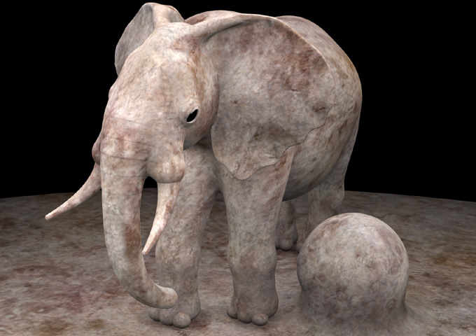
The idea came up during a talk I was giving when somebody asked whether there exists an efficient method to apply textures to models which don't come with uv-coordinates. This can happen for meshes that haven't been UV-mapped yet, or for 3D objects that are not based on meshes or polygons, such as implicit SDFs functions (like the elephant above). The person asking was in particular interested in some alternative to triplanar texture mapping that would be cheaper in terms of number of texture fetches. So I proposed exploring whether some modification could be done that does conditional texturing fetching. Later that night at home I tried the idea myself to see if it would actually work. And it did. This article is about that, but first let's quickly recap what "triplanar mapping" is.

Box/RoundCube/Triplanar mapping

---

This is an ancient but still very useful and simple technique to apply textures to models that aren't or can't be uv-mapped. When the texture to be applied can be described procedurally, such uv-less models are often textured with 3D textures - simply feeding the surface's position coordinates into the procedural texture's input works beautifully. One trick that I think not that many people are aware of however is that these kind of 3D textures DO support model animation easily - all you need to do is use the position of the surface in its reference pose as input to the texture (these reference vertex positions are called "the Pref channel" in Renderman/Pixar for example).

Anyways, when the texture cannot be easily created procedurally by the artists in the team, traditional and easily authored 2D texture bitmaps need to be employed. For some shapes simple things like planar projections, cylindrical projections, spherical projections or octahedral projections will do fine, but except a few models that resemble those base shapes, those projections don't work well for general models and produce stretched textures.

So this is where multi-projections come in. Instead of having a single projection for the whole model, we allow multiple projections to coexist such that they complement each other. This means that where one projection starts to fail because there's too much stretching, another projection can take over.

The easiest way to see this is with planar projections, where they work great for surfaces in the model that are parallel to the projection plane, ie perpendicular to the projection direction, but fail miserably on surfaces that are perpendicular to the projection plane because they create long stripes of color since one of the rate of change of one of the texture coordinates is too small. You've probably seen this in the movie Interstellar, or more probably along the cliffs of a terrain model that you have texture mapped with a simple 2D projection (say using the two non-vertical coordinates of the model vertices as uv coordinates).

One way to assign multiple projections for our model is to define them by hand. Pixar had a tool to do this called Picasso, which was very powerful. But also laborious for the artists. But a compromise exists where one performs automatic multi-projections at the cost of not being so powerful.

That's why Mitch Prater invented the RoundCube texture mapping in the early 90s. If you are a game developer you might only have been exposed to his technique much more recently, under the name of "triplanar" mapping. The idea is simple - just fix the three projection directions to be the canonical directions of space, X, Y and Z. Then color blend the result of the three projection mappings based on how parallel the surface is to each one of those projections, in order to smoothly let the best projections of the three (the most parallel one) take over the other two.

This can be done super easily with a dot product of the surface normal and the X, Y, Z axis vectors, which naturally reduces to simply considering the appropriate X, Y or Z component of the normal and using it to determine the weight of the corresponding projection.

The weight is usually this dot product raised to a positive integer power, such that the influence of each projection sticks to the surfaces parallel to them for a longer time. The result is that you get a weighting function that intuitively feels like a rounded cube, hence the "RoundCube" name that Mitch gave to the technique thirty years ago and which still survives to this day in the Renderman documentation.

The code is naturally super simple and you've seen it many times by now, but just in case, here you can find a live GLSL implementation: https://www.shadertoy.com/view/MtsGWH:

Biplanar mapping

---

So, returning to the original question - how to make this technique more performant? Since reading textures is very costly relative to performing arithmetic and logic operations, a natural thing to try is to reduce the number of texture fetches from three to two. And the simplest way to accomplish that is to pick the two most relevant of the three canonical projections and work with them while completely disregarding the third one. Let me show you the code first and let's discuss it afterwards because there are a couple of interesting things to unpack in the technique (live GLSL implementation here: https://www.shadertoy.com/view/ws3Bzf):


So, first of all, the routine is much longer. But don't let that fool you into thinking is more expensive - while there is some ALU work (logic), there are only two texture fetches, and much of the visual complexity comes from the fact that we have to provide texture gradient by hand. But one thing at a time.

The most important thing this function does is to pick which two of the three projections are the most aligned to the surface we are texturing. Finding the most aligned one, what I called the "major axis", is pretty trivial - just compare the X, Y and Z components of the normal to each other, and whichever is the largest (in absolute value) indicates which one of the three projections X, Y or Z is the most parallel to the surface. This can be done easily with just a few comparisons.


These comparisons are most likely compiled to conditional moves rather than actual branches. I store the index of the largest projection in the first component of the "ma" variable. If ma.x is 0, it means the largest projection is along the X axis, if the value is 1 it references the Y axis and if it's 2 it is the Z axis. The second and third components of the "ma" varible store the "other two" axis which are not major, in lexicographic order, which is important for getting proper planar texturing.

Finding the minor axis, or the worst of the three projections, is equally trivial: finding the smallest of the three coordinates tells us which projection is less parallel to the current surface point that we are texturing. It is stored in the "mi" variable.


Now, how to easily find the median axis, or the second best (or second worst) projection, is maybe not so obvious at first glance. But by excluding the major and minor axis, what we are left with is necessarily the median one, since we only have three. We'll store it in the variable "me", and performing the operation me = 3-ma-mi will give us the desired second best axis. This is because whichever values in {0,1,2} the major and minor axis took, the addition of the three axis indices must be 3, since 0+1+2=3. So 3-ma-mi will disclose which axis was the median one. If this doesn't feel terribly intuitive to you, no worries, it takes a minute of pen and paper doodling to see why this works.


Once the two best projection axis have been determined and stored in the first components of "ma" and "me", together with their following lexicographic axis indices in the second and third components of these variables, all that is left to do is what we have always done in trilinear mapping, but with only two projections rather than three. That is, perform the two texture fetches, and then compute the linear combination of their colors. So let's do those fetches first:


Now, this code above alone can produce artifacts, because the selection of the two closest projections is not a smooth function of the surface normal, but a discontinuos one - it sometimes happens abruptly. Indeed those conditional moves will produce big jumps in the values of "p", and that will confuse the mipmapping algorithm inside the texture sampler. So, we can avoid the discontinuities by taking the gradients of "p" before we do the axis selection, and then pass the appropriate components of those gradients to the texture sampling function.


Without providing the gradients manually, the bilinear mapper will produce the typical one-pixel wide line artifacts seen in most bugs related to mipmapping.

The last bit of code worth mentioning is the construction of the local support through a linear remapping of the weights. If the line


wasn't implemented, we'd have some (often small) texture discontinuities. These discontinuities would naturally happen in areas where the normal points in one of the eight (±1,±1,±1) directions. This happens because at some point the minor and median projection directions will switch places and one projection will be replaced by another one. In practice with most textures and with most blending shaping coefficients "l", the discontinuity is difficult to see, if at all, but the discontinuity is always there. Luckily it's easy to get rid of it by remapping the weights such that 1/sqrt(3), 0.5773, is mapped to zero.

Now, this height remapping removes the discontinuity but narrows the blending areas considerably, so the look of a biplanar mapper is closer to a triplanar mapping with an aggressive blending factor of "k" equal to 8. Because of that you'll find a division by 8.0 in the code I propose for the biplanar mapper, because that makes the biplanar texture mapper an visually satisfactory replacement for the triplanar mapper.

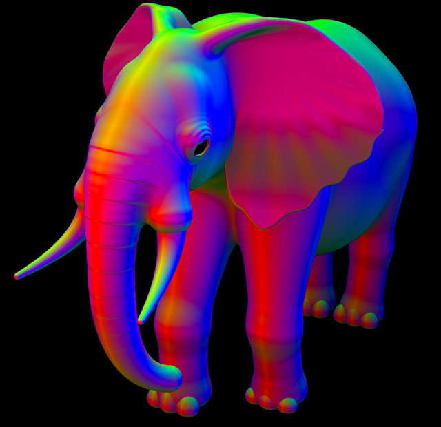
Triplanar, k=1

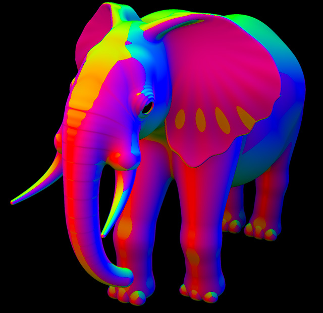
Biplanar, k=8, no remapping

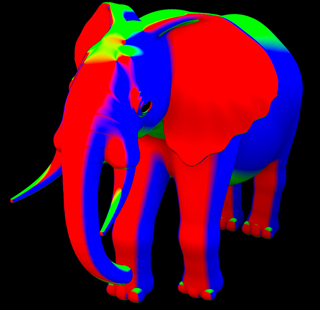
Biplanar, k=1 with local support (remapping)

Triplanar, k=8

Note how biplanar and triplanar mapping look very similar, except near the singularities produced when the normal points towards (±1,±1,±1). A couple of them can be clearly seen in the pictures above on the head of the elephant where red, green and blue meet abruptly.

Another alternative to the remapping is to simply skip it but then only use high values of "k", which will reduce the weight of the least relevant projection to zero quickly. For example, with "k"=8, we get 1/sqrt(3)⁸ = 0.012 = 1.2%, which is small enough that in practice it will be totally unnoticeable.

Testing it

---

This implementation of biplanar mapping works surprisingly well. I'd definitely use it in situations where fetching textures is a bottleneck for the renderer. It is a direct replacement to the triplanar mapper, so it really costs nothing to give it a try and see how it goes for your application.

Here's a closeup comparison of biplanar vs triplanar mapping, focused in the singularity areas for the elephant model:


Biplanar vs Triplanar mapping, near singularities


This is a real time demonstration of the biplanar mapping technique in action in Shadertoy (https://www.shadertoy.com/view/ws3Bzf) - press the Play button to see in animated:



And finally, here's a video that summarizes a bit some of the things we've talked about in this article and a live GLSL implementation at https://www.shadertoy.com/view/3ddfDj):


Biplanar texture mapping video

Related ideas

---

When I published this article a couple of people shared with me other ideas they had to reduce the cost of triplanar mapping, so I'll share them here too:

Nicholas Brancaccio proposed the stochastic route, which is always a valid route if the variance of your Montercarlo rendered image is coming from somewhere other than the surface textures (and probably is). So, simply get ready to do triplanar texture mapping as usual but pick just one of the three projections at random. Of course you can get the random sample from a distribution that is proportional to the weights of the three projections and skip the blending altogether. This might even work fine in realtime applications if you are already heavily dithering lots of the visual elements of the image and are doing some temporal reprojection to smooth things out.

There's another idea that is almost identical to the one in this article which Chris Green from Valve said was used in the "Half Life 2 Ep 2" game. It's this one: skip the detection of the most important projections, and instead prepare to do regular triplanar mapping. However, apply a weight remapping like the one we have in this article, such that we create a more local support and the least important projection's weight becomes zero. Then, for each one of the three projections check if the weights is above zero, and only if it is do the conditional texture fetch. Most times this will result in only two of the three textures being sampled, except for a few regions of the model where the three will still be sampled. The advantage is that it has a bit less ALU involvement, but the disadvantage is that conditionally sampling textures can be a problem in some architectures. On the other hand, the cost of the ALU in the implementation in this article probably is quickly offset in real scenarios by the cost of the multiple texture fetches needed to support albedo, normal map, roughtness, etc.